
| 일 | 월 | 화 | 수 | 목 | 금 | 토 |
|---|---|---|---|---|---|---|
| 1 | 2 | 3 | ||||
| 4 | 5 | 6 | 7 | 8 | 9 | 10 |
| 11 | 12 | 13 | 14 | 15 | 16 | 17 |
| 18 | 19 | 20 | 21 | 22 | 23 | 24 |
| 25 | 26 | 27 | 28 | 29 | 30 | 31 |
- kmu
- 프로그래머스
- GIT
- 스택
- 머신 러닝
- programmers
- Heap
- 회귀
- SQL
- Stack
- PANDAS
- 국민대학교
- 국민대
- gan
- db
- machine learning
- 재귀
- Regression
- instaloader
- python3
- Seq2Seq
- LSTM
- Python
- C++
- 운영체제
- OS
- 데이터베이스
- 파이썬
- googleapiclient
- 정렬
- Today
- Total
정리 노트
CNN with Pytorch 본문
CNN의 개념을 알고 싶은 분들은 제가 저번에 적어놓은 글을 읽어보셔도 됩니다.
CNN이란 무엇인가? 2022.08.29 - [개념 정리/머신러닝 & A.I] - CNN(Convolutional Neural Network)
여기서 작성된 코드는 거의 Pytorch 사이트에 있는 코드입니다. 코드는 Google Colaboratory 기준으로 작성했습니다.
https://pytorch.org/tutorials/beginner/blitz/cifar10_tutorial.html
Training a Classifier — PyTorch Tutorials 1.13.0+cu117 documentation
Note Click here to download the full example code Training a Classifier This is it. You have seen how to define neural networks, compute loss and make updates to the weights of the network. Now you might be thinking, What about data? Generally, when you ha
pytorch.org
저희가 만들 CNN에 학습시킬 데이터는 CIFAR10 데이터셋으로 torchvision 패키지에서 제공합니다.
1. 데이터 정규화
torchvision 데이터셋의 출력은 [0, 1] 범위 안의 값을 가지는 PIL 이미지이기 때문에 이를 [-1, 1] 범위 안의 값을 가지는 Tensor로 변환합니다.
import torch
import torchvision
import torchvision.transforms as transforms


transform = transforms.Compose(
    [transforms.ToTensor(),    # Tensor로 변환

     # 채널 별로 mean = (0.5, 0.5, 0.5), std = (0.5, 0.5, 0.5)로 정규화
     transforms.Normalize((0.5, 0.5, 0.5), (0.5, 0.5, 0.5))]
)

# 데이터셋 다운로드 및 DataLoader로 변환
trainset = torchvision.datasets.CIFAR10(root='./data', train=True,
                                        download=True, transform=transform)
trainloader = torch.utils.data.DataLoader(trainset, batch_size=4,
                                          shuffle=True, num_workers=2)

testset = torchvision.datasets.CIFAR10(root='./data', train=False,
                                       download=True, transform=transform)
testloader = torch.utils.data.DataLoader(testset, batch_size=4,
                                         shuffle=False, num_workers=2)

# 총 10개의 클래스를 가지고 있는 데이터셋입니다.
classes = ('plane', 'car', 'bird', 'cat', 'deer', 'dog', 'frog', 'horse',
           'ship', 'truck')
2. CNN 모델 정의
Convolution, Pooling, Fully Connected 레이어들과 활성화 함수를 정의합니다.
import torch.nn as nn
import torch.nn.functional as F
class CustomCNN(nn.Module):
def __init__(self):
super().__init__()
self.conv1 = nn.Conv2d(3, 6, 5) # input_channel: 3, output_channel: 6, kernel_size: 5
# After convolution -> output size: (32 - 5 + 2 * 0) / 1 + 1 = 28
self.pool = nn.MaxPool2d(2, 2)
# After pooling -> output size: 14
self.conv2 = nn.Conv2d(6, 16, 5)
# After convolution -> output size: (14 - 5 + 2 * 0) / 1 + 1 = 10
# After pooling -> output size: 5
self.fc1 = nn.Linear(16 * 5 * 5, 120)
self.fc2 = nn.Linear(120, 84)
self.fc3 = nn.Linear(84, 10)
def forward(self, x):
x = self.pool(F.relu(self.conv1(x)))
x = self.pool(F.relu(self.conv2(x)))
x = x.view(-1, 16 * 5 * 5)
x = F.relu(self.fc1(x))
x = F.relu(self.fc2(x))
return self.fc3(x)
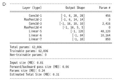
my_cnn = CustomCNN().to("cuda") # GPU에 모델을 올립니다.저희가 설계한 모델의 shape들을 간단하게 볼 수 있는 방법이 있습니다. (이 코드는 위에 걸어둔 링크에 없는 코드입니다.)
import torchsummary

# 간단하게 모델의 shape 살펴보기
torchsummary.summary(my_cnn, (3, 32, 32))
코드를 실행하면 아래와 같이 이쁘게 출력됩니다.
3. 손실 계산, 최적화 방법 정의 그리고 학습
여기서는 CrossEntropyLoss를 손실 함수로 쓰고 Stochastic Gradient Descent 방법으로 최적화를 진행할 것입니다. 이들은 pytorch에서 제공해주기 때문에 손으로 직접 구현할 필요 없이 가져다 쓰면 됩니다.
import torch.optim as optim

criterion = nn.CrossEntropyLoss().to("cuda")
optimizer = optim.SGD(my_cnn.parameters(), lr=0.001, momentum=0.9)
결과를 빠르게 확인하기 위해 epoch을 10만 설정하겠습니다.
for epoch in range(1, 11):
    running_loss = 0.0
    for i, data in enumerate(trainloader, 1):
        inputs, labels = data

        optimizer.zero_grad()    # gradient 초기화
        outputs = my_cnn(inputs.to("cuda"))
        loss = criterion(outputs, labels.to("cuda"))
        loss.backward()    # 역전파 실행
        optimizer.step()    # 최적화 실행

        running_loss += loss.item()
        if i % 2000 == 0:
            print("[%d, %5d] loss: %.3f" % (epoch, i, running_loss / 2000))
            running_loss = 0.0

print("Finish Training.")
학습한 결과는 사리지지 않게 잘 저장합니다.
PATH = './CNN_CIFAR10.pth'
torch.save(my_cnn.state_dict(), PATH)
4. 테스트 셋과 결과 비교
먼저 테스트 셋의 데이터들을 확인해봅시다.
import numpy as np
import matplotlib.pyplot as plt


def imshow(img):
    img = img / 2 + 0.5    # unnormalize
    npimg = img.numpy()    # numpy 배열로 변환
    plt.imshow(np.transpose(npimg, (1, 2, 0)))
    plt.show()

dataiter = iter(testloader)
images, labels = next(dataiter)
imshow(torchvision.utils.make_grid(images))
print(' '.join(f'{classes[labels[j]]:5s}' for j in range(4)))    # Batch size: 4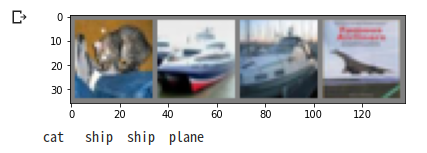
저희가 설계한 모델이 잘 맞췄는지 확인해봅시다.
# 저장한 모델 불러오기
net = CustomCNN()
net.load_state_dict(torch.load(PATH))

outputs = net(images)
_, predicted = torch.max(outputs, 1)
print("Predicted:", ' '.join(f'{classes[predicted[j]]:5s}' for j in range(4)))

# 출력 결과
# Predicted: cat   car   ship  plane
저 같은 경우는 완벽하게 다 맞추지 못했습니다. 모든 테스트 데이터셋에 대해 정확도를 봅시다.
correct, total = 0, 0
with torch.no_grad():    # Training을 하는 것이 아니기 때문에 Gradient들을 계산할 필요 X
    for data in testloader:
        images, labels = data
        outputs = net(images)
        _, predicted = torch.max(outputs, 1)

        total += labels.size(0)
        correct += (predicted == labels).sum().item()
print(f"Accuracy on the 10000 test images: {100 * correct // total} %")

# 출력 결과
# Accuracy on the 10000 test images: 61 %
10개의 클래스들 중 하나를 무작위로 뽑는 것보다는 높은 정확도지만, 개인적으로 만족하지 못하는 정확도입니다...
정확도를 높여보고 싶은 분들은 SGD의 파라미터 값들을 바꾸거나 저희가 설계한 CNN의 깊이를 깊게 해 보는 등 여러 방법들이 있으니 해보시길 바랍니다.
이 모델이 어떤 클래스를 잘 맞추고 어떤 클래스를 잘 못 맞추는지 확인해봅시다.
correct_pred = {classname: 0 for classname in classes}
total_pred = {classname: 0 for classname in classes}

with torch.no_grad():
    for data in testloader:
        images, labels = data
        outputs = net(images)
        _, predicted = torch.max(outputs, 1)

        for label, prediction in zip(labels, predicted):
            if label == prediction:
                correct_pred[classes[label]] += 1
            total_pred[classes[label]] += 1

for classname, correct_count in correct_pred.items():
    accuracy = 100 * float(correct_count) / total_pred[classname]
    print(f"Accuracy for class: {classname:5s} is {accuracy:.1f} %")

# 출력 결과
# Accuracy for class: plane is 71.8 %
# Accuracy for class: car   is 77.4 %
# Accuracy for class: bird  is 41.3 %
# Accuracy for class: cat   is 44.2 %
# Accuracy for class: deer  is 53.2 %
# Accuracy for class: dog   is 46.5 %
# Accuracy for class: frog  is 77.0 %
# Accuracy for class: horse is 71.9 %
# Accuracy for class: ship  is 72.3 %
# Accuracy for class: truck is 62.9 %
출력된 내용을 보면 car 클래스를 가장 잘 맞췄고, bird 클래스에 대해 저조한 성적을 냈음을 알 수 있습니다.
'구현' 카테고리의 다른 글
| AlexNet with Pytorch (0) | 2022.12.04 |
|---|
